Dynamic Model for Macroeconomics in Medium Run
In the dynamic AD-AS model, we remove the assumption that the inflation rate, the expectation for the inflation rate and output growth are zero in the medium run. Additionally, we had assumed that there is no growth in the medium run. This implies that the size of the economy is fixed in the medium run. More realistic is to allow output to trend up over time, for the economy to grow. Thus, the model will now explain all of the business cycle allowing for a trend in income.

So, beforehand we need to be more precise when discussing the policy changes, we need to separate the effects of the real interest rates and the nominal interest rates and how inflation expectations are formed.
PHILLIPS CURVE
AS curve: P = P_e (1+mew)F(u,z)
Assuming the function F and substituting,
P(t) = P_e(t)(1+mew)(1-au(t)+z),
where a is a parameter. In the static model we had assumed that prices come back to a certain level and remain there, that is, inflation in the medium run is zero. But in this model we will allow for prices to change in the medium run, therefore, the equation in terms of inflation rates becomes,
pi(t) = pi_e(t) + (mew+z) - au(t), that is,

pi(t) - inflation at time t
pi_e(t) - expected inflation
u(t) - unemployment in year t
mew and z are assumed constant
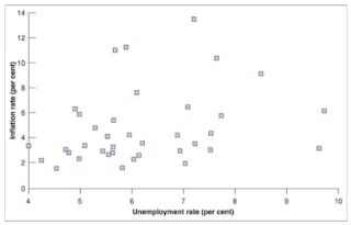
The inflation versus the unemployment data in the USA from 1900-1960 suggested a negative relation between inflation and unemployment.

So, in the Phillips curve is given by the following equation,
pi(t) = pi_e(t) + (mew+z) - au(t), the natural rate of unemployment is given by, u(n) = (mew+z)/a
Phillips Curve - Version-1: Static Expectations
P_e(t) = P(t-1),
therefore, pi_e(t) = 0
or, in words, the inflation expectations are zero. Then the phillips curve becomes,
pi(t) = (mew+z) - au(t), that is,

This is the negative relationship between unemployment and inflation that was found by Phillips for the UK and Solow and Samuelson for the US.
This equation leads to the wage-price spiral, which can be used to an extent to understand the race between prices and the wages resulting in steady wage and price inflation in those periods,
1. Low unemployment leads to a higher nominal wage
2. In response to the higher nominal wage, firms increase their prices and the price level increases
3. In response, workers ask for a higher wage
4. Higher nominal wage leads firms to further increase the prices. As a result, the prices increase further.
Phillips Curve - Version-2: Expectations-Augmented Phillips Curve

Before the 1970s, since the inflation was low and not very persistent, so it was reasonable for workers and firms to ignore past inflation, therefore, pi_e(t) = 0. But as inflation became more persistent, workers and firms started changing the ways they formed expectations. They started looking at past inflation to predict current inflation.
Therefore, the negative relationship between unemployment and inflation had vanished mainly due to two reasons:
1. Price of oil, but more importantly,
2. A change in the way wage setters formed expectations due to a change in the behaviour of the rate of inflation. This period was marked with inflation becoming persistent and positive.
Such changes in expectations formation altered the nature of the relationship linking unemployment and inflation.
So, now the expectations of inflation were formed according to a backwards-looking rue (adaptive expectations rule)
pi_e(t) = theta*pi(t-1)
The parameter theta captures the effect of last years inflation rate (pi(t-1)) on this year's expected inflation rate (pi_e(t)). It was this value of theta that had steadily increased in the 1970s, from zero to 1.
When theta is zero, we get version 1 of the Phillips curve, that is, the one before the 1970s.
When theta is one, we get version 1 of the Phillips curve, that is, the one after the 1970s.
So, the Phillips curve becomes,
pi(t) - pi(t-1) = (mew+z) - au(t), that is,

This relationship also fits the observation of a clear negative relationship between the unemployment rate and the change in the inflation rate.

Under this scenario, the unemployment rate affects not the inflation rate, but the change in the inflation rate. In other words, not only the increase or decrease in the price level but the rate at which the price level would increase or decrease. Or, for example, low unemployment would result in an increase in the inflation rate and thus an acceleration of the price level. This type of Phillips curve is called the expectations-augmented Phillips curve.
According to version 1 of the Phillips curve, there was a permanent tradeoff between the unemployment rate and inflation. Therefore, before the 1970s, economists believed that if the unemployment rate, then it would lead to an increased inflation rate. So, suppose, if earlier prices were increasing at 2% per year and the unemployment rate decreases by 2% then the prices would increase now by 4% per year (approx) and at this constant rate. However, the newer Phillips curve suggests that if earlier prices were increasing at 2% per year and the unemployment rate decreases by 2% then the inflation rate itself would increase now by 4% and so the prices would increase at an accelerated rate.


Therefore, version 2 of the Phillips curve can be re-written as,

It gives us another way of thinking about the Phillips curve: as a relation between the actual unemployment rate, the natural unemployment rate and the change in the inflation rate. It also gives us another way of thinking about the natural rate of unemployment. The non-accelerating inflation rate of unemployment (NAIRU), the rate of unemployment required to keep the inflation rate constant.


Phillips Curve - Version-3: Rational Expectations
pi_e(t) = pi(t) => u(t) = u(n)
So, under R.E. (perfect foresight), the unemployment rate always equals its natural rate.
Policy Implications:
1. For adaptive (backwards looking) expectations, monetary policy may temporarily affect the unemployment rate. This is since the conducted monetary policy would determine the past inflation rates, which then would lead to expected inflation rates in the future, which would subsequently decide the unemployment rates.

2. However, for rational (forward-looking) expectations, monetary policy is more limited in its ability to stimulate the economy. In the extreme case of perfect foresight, monetary policy is ineffective.

OKUN's LAW
The relation between the output growth and the change in the unemployment rate is summarised by Okun's law. Using data, the line based on 30 years of US data comes out to be:
u(t) - u(t-1) = -0.4(g(yt) - 3%)
Thus, we see that if the growth rate is above the natural rate then the unemployment would decrease and vice versa. For unemployment to remain constant, output growth must be at 3% per year. This growth rate of output is called the normal growth rate (this will be the long run growth path in the Solow model)
Further, what we observe from Okun's equation is that there is no 1-to-1 relation between the unemployment rate and growth rates. This is mainly because of labour hoarding. Firms prefer to keep workers rather than lay off when output decreases. When employment increases, not all new jobs are filled by the unemployed. So, when the growth rate increases by 1% above the natural rate, there is a 0.6% increase in the employment rate and 0.4% decrease in the unemployment rate.
In general, Okun's law is,


AGGREGATE DEMAND
We assume a linear version of the aggregate demand relation, that is,
Y(t) = gamma*(M(t)/P(t))

Expressing it in terms of the growth rates, g(yt) = g(mt) - pi(t), or,

The growth rate of output equals the growth rate of the nominal money stock minus inflation. So, expansionary monetary policy (nominal money growth is faster than inflation) leads to increased growth rates of output.
Thus, we have discussed the major components of the dynamic model for the medium run.


So, beforehand we need to be more precise when discussing the policy changes, we need to separate the effects of the real interest rates and the nominal interest rates and how inflation expectations are formed.
PHILLIPS CURVE
AS curve: P = P_e (1+mew)F(u,z)
Assuming the function F and substituting,
P(t) = P_e(t)(1+mew)(1-au(t)+z),
where a is a parameter. In the static model we had assumed that prices come back to a certain level and remain there, that is, inflation in the medium run is zero. But in this model we will allow for prices to change in the medium run, therefore, the equation in terms of inflation rates becomes,
pi(t) = pi_e(t) + (mew+z) - au(t), that is,
pi(t) - inflation at time t
pi_e(t) - expected inflation
u(t) - unemployment in year t
mew and z are assumed constant
The inflation versus the unemployment data in the USA from 1900-1960 suggested a negative relation between inflation and unemployment.
So, in the Phillips curve is given by the following equation,
pi(t) = pi_e(t) + (mew+z) - au(t), the natural rate of unemployment is given by, u(n) = (mew+z)/a
Phillips Curve - Version-1: Static Expectations
P_e(t) = P(t-1),
therefore, pi_e(t) = 0
or, in words, the inflation expectations are zero. Then the phillips curve becomes,
pi(t) = (mew+z) - au(t), that is,

This is the negative relationship between unemployment and inflation that was found by Phillips for the UK and Solow and Samuelson for the US.
This equation leads to the wage-price spiral, which can be used to an extent to understand the race between prices and the wages resulting in steady wage and price inflation in those periods,
1. Low unemployment leads to a higher nominal wage
2. In response to the higher nominal wage, firms increase their prices and the price level increases
3. In response, workers ask for a higher wage
4. Higher nominal wage leads firms to further increase the prices. As a result, the prices increase further.
Phillips Curve - Version-2: Expectations-Augmented Phillips Curve
Beginning in the 1970s, the relation between the unemployment rate and the inflation disapparated in the US. Now, we will discuss the reason behind this disappearance.
Post-1960s, the US inflation rate was consistently positive. Inflation had become more persistent: a high inflation rate this year is more likely to be followed by a high inflation rate next year.
Before the 1970s, since the inflation was low and not very persistent, so it was reasonable for workers and firms to ignore past inflation, therefore, pi_e(t) = 0. But as inflation became more persistent, workers and firms started changing the ways they formed expectations. They started looking at past inflation to predict current inflation.
Therefore, the negative relationship between unemployment and inflation had vanished mainly due to two reasons:
1. Price of oil, but more importantly,
2. A change in the way wage setters formed expectations due to a change in the behaviour of the rate of inflation. This period was marked with inflation becoming persistent and positive.
Such changes in expectations formation altered the nature of the relationship linking unemployment and inflation.
So, now the expectations of inflation were formed according to a backwards-looking rue (adaptive expectations rule)
pi_e(t) = theta*pi(t-1)
The parameter theta captures the effect of last years inflation rate (pi(t-1)) on this year's expected inflation rate (pi_e(t)). It was this value of theta that had steadily increased in the 1970s, from zero to 1.
When theta is zero, we get version 1 of the Phillips curve, that is, the one before the 1970s.
When theta is one, we get version 1 of the Phillips curve, that is, the one after the 1970s.
So, the Phillips curve becomes,
pi(t) - pi(t-1) = (mew+z) - au(t), that is,
This relationship also fits the observation of a clear negative relationship between the unemployment rate and the change in the inflation rate.

Under this scenario, the unemployment rate affects not the inflation rate, but the change in the inflation rate. In other words, not only the increase or decrease in the price level but the rate at which the price level would increase or decrease. Or, for example, low unemployment would result in an increase in the inflation rate and thus an acceleration of the price level. This type of Phillips curve is called the expectations-augmented Phillips curve.
According to version 1 of the Phillips curve, there was a permanent tradeoff between the unemployment rate and inflation. Therefore, before the 1970s, economists believed that if the unemployment rate, then it would lead to an increased inflation rate. So, suppose, if earlier prices were increasing at 2% per year and the unemployment rate decreases by 2% then the prices would increase now by 4% per year (approx) and at this constant rate. However, the newer Phillips curve suggests that if earlier prices were increasing at 2% per year and the unemployment rate decreases by 2% then the inflation rate itself would increase now by 4% and so the prices would increase at an accelerated rate.


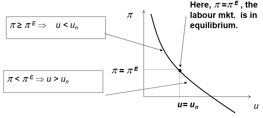
The tradeoff between unemployment and inflation as was suggested by version 1 was argued by Friedman and Phelps, who said that the unemployment rate could not be sustained below a certain level, a level they called the "natural rate of unemployment". This the unemployment rate at which the actual inflation rate is equal to the expected inflation rate ( the medium run).
u(n) = (mew+z)/a that is,
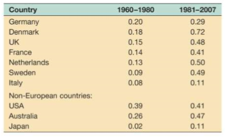
In this equation, the mew and z may not be constant but, in fact, vary over time, leading to changes in the natural rate of unemployment. In Europe, the natural rate has increased a lot since the 1960s. In the US, the natural rate increased by 1-2 percentage points from the 1960s to the 1980s and appears to have decreased since then.
It gives us another way of thinking about the Phillips curve: as a relation between the actual unemployment rate, the natural unemployment rate and the change in the inflation rate. It also gives us another way of thinking about the natural rate of unemployment. The non-accelerating inflation rate of unemployment (NAIRU), the rate of unemployment required to keep the inflation rate constant.
From this equation, we can see that when the unemployment rate exceeds the natural rate of unemployment, the inflation rate starts to decrease. When the unemployment rate is below the natural rate of unemployment, the inflation rate starts to increase.
So, in the short run, the expectations-augmented Phillips curve is downward sloping while in the medium run its vertical.

pi_e(t) = pi(t) => u(t) = u(n)
So, under R.E. (perfect foresight), the unemployment rate always equals its natural rate.
Policy Implications:
1. For adaptive (backwards looking) expectations, monetary policy may temporarily affect the unemployment rate. This is since the conducted monetary policy would determine the past inflation rates, which then would lead to expected inflation rates in the future, which would subsequently decide the unemployment rates.
OKUN's LAW
The relation between the output growth and the change in the unemployment rate is summarised by Okun's law. Using data, the line based on 30 years of US data comes out to be:
u(t) - u(t-1) = -0.4(g(yt) - 3%)
Thus, we see that if the growth rate is above the natural rate then the unemployment would decrease and vice versa. For unemployment to remain constant, output growth must be at 3% per year. This growth rate of output is called the normal growth rate (this will be the long run growth path in the Solow model)
Further, what we observe from Okun's equation is that there is no 1-to-1 relation between the unemployment rate and growth rates. This is mainly because of labour hoarding. Firms prefer to keep workers rather than lay off when output decreases. When employment increases, not all new jobs are filled by the unemployed. So, when the growth rate increases by 1% above the natural rate, there is a 0.6% increase in the employment rate and 0.4% decrease in the unemployment rate.
In general, Okun's law is,
The parameter beta gives the effect of output growth deviations on unemployment rates. It can change across countries and with time.
So, growth above the normal rate would mean that unemployment rates would fall and vice versa.

AGGREGATE DEMAND
We assume a linear version of the aggregate demand relation, that is,
Y(t) = gamma*(M(t)/P(t))
Expressing it in terms of the growth rates, g(yt) = g(mt) - pi(t), or,
The growth rate of output equals the growth rate of the nominal money stock minus inflation. So, expansionary monetary policy (nominal money growth is faster than inflation) leads to increased growth rates of output.
Thus, we have discussed the major components of the dynamic model for the medium run.

SCENARIOS
Assumptions:
1. IS
a. Consumption - Depends on the growth of disposable income
b. Investment - Depends on the growth of income and interest rate
c. Government Expenditure - Exogenous
d. Taxation - Exogenous
e. Net exports - Equal to zero - Closed economy
f. Exchange rate - Not considered - Closed economy
2. LM
a. Money demand - Choice between money and bonds
b. Money supply - Exogenous, growth rate of money supply is positive in the medium run
3. Production function - One type of output and technological change. Depends on labour only, with constant returns to scale. Labour force is not constant.
4. Labout market - Determined by the interaction of wage setting and price setting equations. Expectations of inflation are fixed in the short run
5. Technological change - Exogenous, positive and constant
Now, being equipped with tools, let's discuss some examples.
Example1. Effect of expansionary monetary policy or an increase in money growth.
In the medium run, we know that there is no shock to the output and so it would grow at its normal rate of growth, g_bar. Unemployment will return to its natural level. Expected inflation would be equal to the actual inflation so delta_pi_t would be equal to zero.
However, an increase in the money supply would lead to an increase in inflation. So, we see again that money is neutral and expansionary monetary policy (permanent increase) will have inflationary effects.
Example2. A supply shock hits and increases the natural rate of unemployment. So, in the short run, firstly, inflation would rise. But since the growth rate of output and money supply has not been affected, so in the medium run, inflation would come back to the same level. In the short run, due to increased inflation, the growth rate of output would decrease, which would then come back to the natural level. Due to the decreased growth rate of output, the unemployment rate would increase, finally settling at the new increased natural rate. The response to the monetary policy should be such that it helps attain the newer medium run equilibrium quickly, or the new higher natural rate of unemployment. So, we may suggest a temporary contractionary policy.
Example3. A supply shock hits and increases the natural rate of output. So, the growth rates would rise even in the short run. Now, since the output growth rates have been permanently increased, it would lead to the decreased inflation rate in the medium run. Further, increased growth rates of output in the short run would lead to increased unemployment rates in the short run. However, they would come back to the natural rate in the medium run. Increasing unemployment rates would then lead to decreased inflation in the short run which would set up at the newer lower level.
To know what happens to all the macro variables (consumption, investment etc) we need to know what happens to interest rates as well. Now, there are two types are interest rates, the nominal interest rates and the real interest rates. The real interest rate is (approximately) equal to the nominal interest rate minus the expected rate of inflation.
So, if the expected inflation equals zero, nominal and real interest rates are equal. But if the expected inflation rate is positive,t then nominal interest rates would be greater than the real interest rates.
In the medium run, the real interest rate is determined by the balance between saving and investment opportunities. So, the investment depends on real interest rates. We will assume that it varies only if there are changes to fiscal policy (we will get crowding out from fiscal policy).
Our IS relation transforms to,
While our LM relation remains,
Note an immediate implication of this is that,
1. The interest rate directly affected by monetary policy is the nominal interest rate
2. The interest rate that affects spending and output is the real interest rate
3. So, the effects of monetary policy on output growth in the short run depend on how movements in the nominal interest rate translate into movements in the real interest rate
Policy implications - Monetary policy:
(Permanently) higher money growth leads to a lower nominal interest rate in the short run, but to higher nominal interest rates in the medium run. In the short run, the increase in money growth increases the real money stock which therefore decreases the interest rates (both real and nominal). In the medium run, because the expansionary monetary policy leads to inflation, so according to the equation, delta_i > delta_r such that delta_i = delta_pi(e) (in the long run) which keeps delta_r constant:
Higher money growth rate leads to a lower real interest rate in the short run but the original real interest rate in the medium run. So, the monetary policy does not affect GDP nor its composition (the neutrality of money)
Reducing the IS relation, LM relation and relation between the real and nominal interest rate gives us,
In the medium run, a change in the growth rate of the money supply will lead to a one-for-one increase in the nominal interest rate and inflation. This result is known as the Fischer effect.
So, comparing the dynamic vs static model for monetary policy:
1. In the static model, the monetary policy changes price levels in the medium run but also changes the composition of GDP (since interest rates also change) but not the actual GDP (in the medium run)
2. In the dynamic model, the monetary policy changes prices levels in the medium run neither change the composition of GDP (since real interest rates do not change) nor the actual GDP.
Policy implications - Fiscal policy:
In the medium run, the output growth rate returns to the natural rate and unemployment to the natural rate. The rate of inflation is equal to the rate of money growth minus the rate of growth of the output. The growth rate of C, I, G equal the growth rate of Y in the medium run.
The nominal interest rate changes but so does the real interest rates (because the expected inflation rates do not change). So, the level of investment in the economy changes. So, in the dynamic model, the fiscal policy changes the composition of GDP much like that in the static model.
Further, we will assume that the real interest rate varies only if there are changes to fiscal policy.
But, what we can observe is that the effects of the fiscal and monetary policy which were the same in the static AS-AD are not same in the dynamic model anymore.
The effects of demand shocks and the supply shocks have different effects on the levels of GDP. The slope of the line is g(a), that is, growth of technological progress. Further, we observe that the demand shocks have a temporary effect on the levels of GDP but supply shocks alter the level of GDP.
DISINFLATION
We know that lower inflation requires lower money growth. We also know that lower money growth implies an increase in unemployment for some time. Now we will discuss at what pace the central bank should proceed.
In the Phillips curve relation above, disinflation - a decrease in inflation can be obtained only at the cost of higher unemployment. A point-year of excess unemployment is a difference between the actual and the natural unemployment rate of one percentage point for one year.
For example, let's assume that alpha = 1. Suppose the central bank wants to achieve the reduction in inflation in one year, then one year of unemployment at 10% above the natural rate is required. Suppose the central bank wants to achieve the reduction over 2 years, then 2 years of unemployment at 5% above the natural rate is required. By the same reasoning, reducing inflation over 10 years requires 10 years of unemployment at 1% above the natural rate.
LUCAS CRITIQUE
The dynamic AS-AD model so far assumes adaptive expectation. The Lucas critique states that it is however unrealistic to assume that wage setters would not consider changes in policy when forming their expectation (they would include their expectations of the future). If wage setters could be convinced that inflation was indeed going to be lower than in the past, they would decrease their expectations of inflation, which would, in turn, reduce actual, without the need for a change in the unemployment rate. This comes from the Phillips curve. So, if you need to change inflation, either you change inflation expectations or you change unemployment rates. So, if expectations change automatically, then you need not require changing the unemployment rates. This is basically the Version-3 of the Phillips curve. If pi_e reduces sufficiently automatically, then pi would reduce subsequently without changing the unemployment rates. Under rational expectations (perfect foresight) there is no tradeoff between inflation and unemployment.
Thomas Sargent, who worked with Robert Lucas, argued that in order to achieve disinflation, any increase in unemployment would have to be only small. So, the essential ingredient of successful disinflation, he argued, was the credibility of monetary policy - the belief by wage setters that the central bank was truly committed to reducing inflation. The central bank should aim for fast disinflation.
NOMINAL RIGIDITIES
A contrary view was taken by Stanley Fischer and John Taylor. They emphasised the presence of nominal rigidities or the fact that many wages and prices are not readjusted when there is a change in policy. If wages are set before the change in policy, inflation would already be built into existing wage agreements. There will be slow adjustment even with forward-looking expectations.
While Fischer argued that even with credibility, too rapid a decrease in nominal money growth would lead to higher unemployment, Taylor's argument went one step further. He argued that wage contracts are not all signed at the same time, but they are staggered over time. He showed that this staggering of wage decisions imposed strong limits on how fast disinflation could proceed without triggering higher unemployment.

In 1993, Laurence Ball, from John Hopkins University estimated sacrifice ratio for 65 disinflation episodes in 19 OECD countries over the last 30 years. He reached three main conclusions:
1. Disinflation typically leads to a period of higher unemployment. (support of Fischer)
2. Faster disinflation is associated with smaller sacrifice ratios. (support of Lucas and Sargent)
3. Sacrifice ratios are smaller in countries that have shorter wage contracts. (support of Taylor)
Comments
Post a Comment