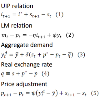
Dornbush Model of Exchange Rates

Unlike Mundel Flemming model, this model introduces dynamics. Further, it takes the role of expectations into account. Dornbusch's model was highly influential because, at the time of writing, the world had recently shifted to a floating exchange rate regime and a little was understood about exchange rate volatilities. It helps us to explain why exchange rates move so sharply from day to day. 

The exchange rate is said to overshoot when its immediate response to a disturbance is greater than its long-run response. Changes in price levels are less volatile, suggesting that price levels change slowly. Exchange rates are influenced by interest rates and expectations, which may change rapidly, making exchange rates volatile.

Assumptions:
1. AD is determined by IS-LM mechanism and therefore, the output is determined by AD
2. Small open economy i.e. foreign interest rates (i*) are exogenous
3. Perfect capital mobility - UIP holds. Investors are risk neutral and domestic and foreign assets are perfect substitutes.
4. Prices are sticky i.e. goods market is sluggish but the forex market shows the quick adjustment.
5. Agents have rational expectations. In the absence of random shocks, they have perfect foresight. Therefore, the expected value of depreciation would equal the actual value of depreciation.

Therefore, we have the following equations for the model,

Note: PPP does not hold in this model. 

Further, equation 5 tells us that in order to keep output at the natural level, nominal exchange rates would change by price differential, however, since prices are sticky nominal exchange rates have to change by larger value to compensate.

Assuming the exogenous values i.e. i*, y_ bar and p* equal 0. Using equations 3,4 and 5 we get,

And using 1,2,3 and 4 we get,

Long run analysis: steady-state lines, 

If q>q_bar then exports rise which leads to relatively higher AD and so y>y_bar. If y>y_bar then prices start to rise which pulls q back towards the steady-state q_bar.

If the slope of s-q line is positive (phi*delta < 1) and the currency depreciates then, output rises, which increases income leading to higher demand for money. Thus, domestic interest rates would increase which would further cause depreciation of currency for UIP to hold. So, we see that the exchange rate movements are amplified because of the UIP condition.

Thus, based on this understanding, the graphical representation of equation 6 and 7 has been shown below

At steady state, i.e. at the intersection of two curves,

If we assume p*=0, then using 4 for the steady-state we get,

So, in the long run, employment is at its maximum level and prices are flexible. Increase in money supply leads to increment in AD since agents will have more funds to spend, which leads to a proportional increase in the price level, leaving with the same real money supply as before. Thus, money is neutral or there is no effect on the real variables in the long run. Further, exchange rates increase to keep real exchange rates at the same level (since q_bar is exogenously given). 

Short run analysis: In the short run because prices are sticky the goods markets adjust slowly, while financial markets adjust instantaneously. The money supply increase shifts the LM to the right, decreasing the interest rate. The increase in M induces a current depreciation of the domestic currency, so the nominal exchange rate increases. Given the interest rate parity, the fall in i must be associated with an expected future appreciation. In order to generate an expected appreciation, the currency overdepreciates (i.e. overshoots) vs. its long-run level. The currency depreciation, together with ΔP = 0 in the short-run, implies that q rises, and IS shifts to the right. The shifts in IS and LM shift aggregate demand, which equals short-run aggregate supply. There is an increase in output produced.  

Then we transition into the long-run equilibrium. Excess aggregate demand pushes up prices. The increased price level reduces real money supply so the LM shifts back to its initial equilibrium. The interest rate rises to its initial position, and as this happens the domestic currency appreciates. The increase in prices, together with the currency appreciation, reduces the domestic economy's competitive advantage in the goods market and IS shifts back to its initial position. We return to the initial real equilibrium with increased prices, A nominal exchange rate depreciation and the real exchange rate at its initial level.

The model exhibits saddle path property. In other words, there exists a unique path along with the economy converges to the long run equilibrium. Saddle path is a curve that shows combinations of all initial conditions from which economy attains equilibrium. It is assumed that the economy is on the saddle path since otherwise, the nominal exchange rate will explode. 

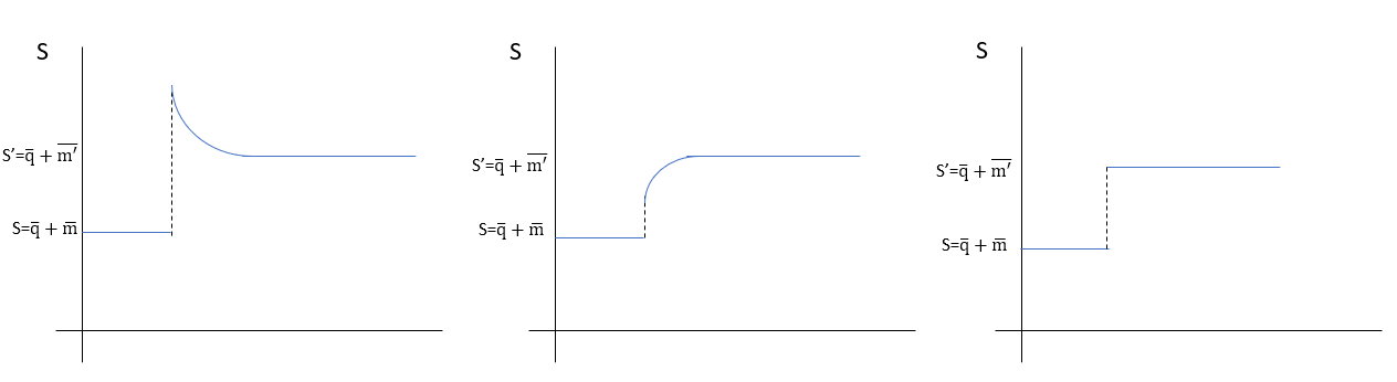
Suppose there is monetary expansion. So,

the nominal exchange rate increases or there is long run depreciation since q_bar is exogenous. Therefore, the new steady state would be above the initial steady state. Increase in the money supply shifts the delta_s = 0 line upwards (look at its equation) and therefore our saddle path is shifted. We have assumed that the economy is always at the saddle path, therefore, the economy will shift from initial equilibrium to somewhere along the shifted saddle path. Now because prices are sticky, q = S - p, change in S leads to an equivalent change in q since p is fixed. So, in the short run, the nominal exchange rate is larger than the new long-run equilibrium for the nominal exchange rate. Thus, fluctuation in the nominal exchange rate is larger than the fluctuation in the money supply. Remember, it was assumed for this analysis that (phi*delta < 1). When phi*delta > 1 then we observe undershooting. It can be understood through equation 2. When phi and delta are small and we have a monetary shock then LHS of equation 2 increases, thus RHS should increase too. If phi*delta is small then i will have to decrease too for increasing RHS further. However, if phi*delta were large then i might even increase, leading to undershooting.

Therefore, if phi*delta:

1. less than 1 => overshooting

2. larger than 1 => undershooting

3. exactly equal to 1 => economy jumps to new equilibrium right away.

The model offers a prediction of a negative correlation between the real exchange rates and real interest rates. Empirical evidence is, for example, the monetary tightening under Thatcher in 1980s.

FOR ESSAY