Intro to Machine Learning and Artificial Intelligence for metricians
There's no clear demarcation between ML, AI, statistics and econometrics. But there are some techniques under ML/AI that are not present in econometrics and could be quite beneficial to adopt.
There are three broad useful principles in the ML/AI way of thinking that would be valuable for econometricians:
1. In econometrics, we don't focus on predictions, but it is a very important part of ML/AI. The commonality between metrics and ML/AI people is that both the sets do agree that there might be tension between the prediction of outcomes and inference on parameters. So, if I focus on prediction, then I might not be able to uncover the underlying structure of the data. Similarly, if I am focusing on having better inference on parameters, I might not be able to have good predictions. Although it might seem counter-intuitive, but there are cases like these as well.
2. Overfitting needs to be kept in mind. Overfitting occurs when we have a better model fit in the sample than in the population. It might occur when we are basically fitting noise in the sample than the signal.
3. There's Bias-Variance tradeoff. This is one of the major lessons to be drawn from ML/AI literature than we can allow for some amount of bias, as it can cut a huge amount of variance.
What is the prediction?
In metrics, so far prediction for us it meant computing Y_hat (equals X*B_hat) using observed data (X). For ML, prediction means supervised learning. Even linear regression is one such, although not a good one. Supervised learning means using X to learn about Y when we have some examples of (X, Y) pairs to discipline and check the learning process. So supervised in the sense that we observe Y. Unsupervised learning is when we use X to learn about Y when we see X but don't see Y.
In ML/AI prediction is the goal and not causal inference, however, it has tools with some minor modifications can help us improve causal inference (which we focus in metrics). The difference between prediction and causal inference however, in recent times has been blurred. In the Neyman Rubin causal model, if we had treated an individual then we would observe Y(1) and not Y(0). But what if we could predict Y(0) very well, in that case, we can compute Y(1) - Y(0) or individual treatment effect. So is it a prediction or causal inference.
In Atlantic Causal Inference Competition fake datasets were produced based on real data sets with known causal structure. The aim was to see which algorithm does better at identifying average treatment effects. They found out (we saw 2018 results) that ML/AI algorithms did much better than econometric models.
There are some features of ML's dominance. One of the reasons was their non-linearity. Also, ML/AI focus on the betterment of out-of-sample performance which we do not discuss in metrics. They also introduce some bias and utilize the bias-variance trade-off concept.
A type of non-linear ML method - Regression Trees. Here we have a regression tree to predict house values with different covariates like bath, rooms etc. The values are predictions (in log($)). What this tree is doing is splitting in a bunch of categorical variables. At each node following command, it cuts continuous variable into smaller bits. In this way, it cuts up covariate space into smaller portions and then makes predictions for Y in this different part of covariate space.

We could represent a tree as the linear regression on dummies for the cuts with leaves being represented as the product of the dummies. Thus, this introduces non-linearity into the structure.
The tree format is very flexible and adding a bunch of trees we can map highly non-linear surfaces. The tree methods outperform linear regression both in predictions and causal inference. But at the same time, isn't being too flexible a problem. Indeed. If our objective were to fit the in-sample data, then using trees we can fit it perfectly. This is because we would then have had split each covariate into N dummy bits and had a different prediction for each data-point. But then ML should be bad. This is because the objective function is not to get a good sample fit. The goal of ML is to have a good out-of-sample prediction. Ex: Google translate - it should not only tell me what words I have trained it with but should recognize new words and predict its translation.
So how does ML optimize for out-of-sample performance - discipline the in-sample fit using,
1. Regularization
2. Cross-validation
Regularization is the act of introducing new information into the prediction problem in order to prevent over-fitting of the sample we have. Its basically like adding a constraint to the model fitting algorithm. In the case of trees, we can think of it as controlling the depth of the tree. Deciding on the depth of the tree (degree of fitting) is called the degree of regularization and can be controlled through the set of parameters called tuning parameters. So, these problems basically constrain the fit of the algorithm within the sample, for us to have a better out-of-sample fit. Thus the right amount of regularization (optimal in-sample-fit so as to have good out-of-sample fit) could be generated by through these tuning parameters. For example, we can have regularization as max(tree depth) = m, where m would be our tuning parameter.
Tuning parameters can take different values depending on the amount of regularization that we want. In our tree example, if we want high regularization then we would set a lower m. So, how can pick good values of tuning parameter which optimize the out-of-sample fit?
Cross-validation is a methodology that allows us to choose tuning parameters. It uses the sample data to select the tuning parameter for us. It splits entire data into a training sample and testing sample. Training sample is one where the model is initially fit. Testing sample is the one which is not involved in fitting but only checking the degree of fit outside the training sample. Similar to the bootstrap mentality, the fit in the training sample would be considered as the fit to population.

In order to do cross-validation, we need to first decide how much data to use to train and how much to test. There are many different ways to do this. Example - Leave-One-Out-Cross-Validation (leaves 1 data-point out, fit on N-1 data-points and then predict the left data-point. Cycle through until all N data-points have been left out once and predicted and then take an average of how well the predictions were made). K-fold cross-validation (splits data into K chunks, leaves 1 chunk out for testing sample and trains on K-1 chunks and similarly cycles through the chunks). Currently, this K is chosen arbitrarily. It should be noted however that cross-validation is simply a procedure and similarly has errors in the finite sample.
All the estimators that we deal with in metrics (OLS, MLE, GMM) are not regularized at all. Because of this, these estimators have higher RMSE than their regularized counter-parts, which would, therefore, outperform the conventional estimators. It is good to keep in mind that OLS is BLUE but in the class of unbiased estimators. Regularization introduces bias. Unbiased estimators often perform very badly in terms of RMSE but in metrics somehow we focus only on them. In ML's perspective, however, its instance because by allowing little bias one can cut down a lot of variances.
ML for Panel data: As a result of the incidental parameters problem, the alpha_i were unbiased but had large variance which made it inconsistent. Thus we could not study individual treatment effects. The problem worsen when we had non-linear models. We can use the ML idea here to regularize estimates of the alpha_i's, thereby introducing bias but cutting down variance.
ML for Non-linear Fixed effects: In non-linear models with fixed effects, we can drop them out only if we know the sufficient statistics. But complex models might not have sufficient statistics or it might be difficult to find. In such cases, we should understand the problem with alpha_i's inconsistency was that I wasn't learning about alpha_i's (fixed effects) as data increases. So I need to learn about alpha_i. We can actually put up a model on alpha_i that creates a sufficient statistic like alpha_i ~ g(X_i, gamma). Suppose, alpha_i ~ N(mew*X_i, sigma_sqaure). So now we can condition on mew and sigma_square to factorize out alpha_i (would work since mew and sigma_square characterize alpha_i). Also, mew and sigma_square can be consistently estimated from the sample.
This is related to an idea called Empirical Bayes. It creates a kind of correlated random effects where data Y is distributed as function f, while FE is distributed as function g. We then condition data on parameters and integrate out FE.

A correlated random effect is a subset of Empirical Bayes idea. The latter is more general in the way that it says to fit the data (distribution) to alpha_i's that depends on the parameters. So, if g function were N(mew, sigma_sqaure). The estimators that we obtain by adding this g() component to any model that we had studied are called as shrinkage estimators. This is because they shrink different alpha_i's towards single mew. The method is Bayes because we can think of g() as the prior distribution of alpha_i if one were a Bayesian.
But we can see that in Empirical Bayes we assume alpha_i's are not correlated with X_i's, which is not right with fixed effects issue. But this works because this assumption invokes bias-variance trade-off. So, we know that it would be biased, but then it will cut down variance. We know that assuming a specific distribution is wrong and will introduce bias because it is basically containing the alpha_i's to be in the proximity of the mean of the defined distribution (if g ~ N(mew, sigma_square then alpha_i's would be supposed to have a common mean, thus restricted). What we want are good wrong models. We won't mind models wrong, but we want them to be useful.
Suppose we don't have much data or variation or too large a covariate dimension to estimate the parameters in the regression. Under such scenarios, we have seen that parameters estimation might result in high variance. We can thus utilize regularization and shrinkage concepts. Suppose we have a model,
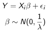
Basically, we are shrinking estimates towards zero or restricting beta to be in the neighbourhood of zero (thus beta would be a weighted average of OLS estimate and zero). But how much freedom to give to beta for it to wander off from zero or the degree of regularization (the second equation which constraints) of beta is decided by the tuning parameter lambda. For example, if lambda were100,000 then all beta's would be near zero, but if lambda were 0.001 then beta's could be moving around a lot and might just be same as the OLS estimates. The mentioned example is called Ridge regression.
In entrepreneurial talent model, each individual had its own beta_i. In cross-section data, we cannot identify beta_i. In the panel we can, but each beta_i is estimated of T data points (which is inconsistent if T is small). Now, what we can do is have these beta_i's in the model but shrink them together.

Shrinkage makes it a homogeneous model where everyone's beta is the same. So we are compromising our original correct but high variance model by saying that everyone has their own beta_i but they all have a common mean. beta and we will shrink beta_i's towards beta using the variance. We can also estimate the variance. So, data itself could tell us how much shrinkage we should do via how much variation it detects in beta_i's distribution. This method would be an Empirical Bayes. If we want to do full Bayes then we will have to assume prior on beta and sigma square which will give us more regularization (more restrictions through more equations, that is for beta and sigma_sqaure). Mixing the unconstrained model (correct but high variance) with the constrained model (incorrect but low variance) would give us the best of both worlds.
Although it might look like we are adding more structure, but actually we are not as shrinkage is containing the parameters too. So we end up having fewer effective parameters. But this also creates a problem since now our effective parameters depend on our tuning parameter (like sigma_square). If we have high sigma_square then no shrinkage and effective parameters might be larger than before. But if we have low sigma_sqaure then there's high shrinkage and low effective parameters. If we are using empirical Bayes then our data tells us the value of sigma square, so there's no way a prior to knowing the effective degrees of freedom.
Another good aspect of regularization which attracts people to use it is that it can make ill-posed problems solvable by reducing the effective number of parameters. Suppose we can't fit OLS because rank(X'X) = N < K, thus overfitting problem. Using regularization we can reduce the effective number of covariates and work.
This is based on the lecture by Dr. Rachael Meager, LSE
There are three broad useful principles in the ML/AI way of thinking that would be valuable for econometricians:
1. In econometrics, we don't focus on predictions, but it is a very important part of ML/AI. The commonality between metrics and ML/AI people is that both the sets do agree that there might be tension between the prediction of outcomes and inference on parameters. So, if I focus on prediction, then I might not be able to uncover the underlying structure of the data. Similarly, if I am focusing on having better inference on parameters, I might not be able to have good predictions. Although it might seem counter-intuitive, but there are cases like these as well.
2. Overfitting needs to be kept in mind. Overfitting occurs when we have a better model fit in the sample than in the population. It might occur when we are basically fitting noise in the sample than the signal.
3. There's Bias-Variance tradeoff. This is one of the major lessons to be drawn from ML/AI literature than we can allow for some amount of bias, as it can cut a huge amount of variance.
What is the prediction?
In metrics, so far prediction for us it meant computing Y_hat (equals X*B_hat) using observed data (X). For ML, prediction means supervised learning. Even linear regression is one such, although not a good one. Supervised learning means using X to learn about Y when we have some examples of (X, Y) pairs to discipline and check the learning process. So supervised in the sense that we observe Y. Unsupervised learning is when we use X to learn about Y when we see X but don't see Y.
In ML/AI prediction is the goal and not causal inference, however, it has tools with some minor modifications can help us improve causal inference (which we focus in metrics). The difference between prediction and causal inference however, in recent times has been blurred. In the Neyman Rubin causal model, if we had treated an individual then we would observe Y(1) and not Y(0). But what if we could predict Y(0) very well, in that case, we can compute Y(1) - Y(0) or individual treatment effect. So is it a prediction or causal inference.
In Atlantic Causal Inference Competition fake datasets were produced based on real data sets with known causal structure. The aim was to see which algorithm does better at identifying average treatment effects. They found out (we saw 2018 results) that ML/AI algorithms did much better than econometric models.
There are some features of ML's dominance. One of the reasons was their non-linearity. Also, ML/AI focus on the betterment of out-of-sample performance which we do not discuss in metrics. They also introduce some bias and utilize the bias-variance trade-off concept.
A type of non-linear ML method - Regression Trees. Here we have a regression tree to predict house values with different covariates like bath, rooms etc. The values are predictions (in log($)). What this tree is doing is splitting in a bunch of categorical variables. At each node following command, it cuts continuous variable into smaller bits. In this way, it cuts up covariate space into smaller portions and then makes predictions for Y in this different part of covariate space.
We could represent a tree as the linear regression on dummies for the cuts with leaves being represented as the product of the dummies. Thus, this introduces non-linearity into the structure.
The tree format is very flexible and adding a bunch of trees we can map highly non-linear surfaces. The tree methods outperform linear regression both in predictions and causal inference. But at the same time, isn't being too flexible a problem. Indeed. If our objective were to fit the in-sample data, then using trees we can fit it perfectly. This is because we would then have had split each covariate into N dummy bits and had a different prediction for each data-point. But then ML should be bad. This is because the objective function is not to get a good sample fit. The goal of ML is to have a good out-of-sample prediction. Ex: Google translate - it should not only tell me what words I have trained it with but should recognize new words and predict its translation.
So how does ML optimize for out-of-sample performance - discipline the in-sample fit using,
1. Regularization
2. Cross-validation
Regularization is the act of introducing new information into the prediction problem in order to prevent over-fitting of the sample we have. Its basically like adding a constraint to the model fitting algorithm. In the case of trees, we can think of it as controlling the depth of the tree. Deciding on the depth of the tree (degree of fitting) is called the degree of regularization and can be controlled through the set of parameters called tuning parameters. So, these problems basically constrain the fit of the algorithm within the sample, for us to have a better out-of-sample fit. Thus the right amount of regularization (optimal in-sample-fit so as to have good out-of-sample fit) could be generated by through these tuning parameters. For example, we can have regularization as max(tree depth) = m, where m would be our tuning parameter.
Tuning parameters can take different values depending on the amount of regularization that we want. In our tree example, if we want high regularization then we would set a lower m. So, how can pick good values of tuning parameter which optimize the out-of-sample fit?
Cross-validation is a methodology that allows us to choose tuning parameters. It uses the sample data to select the tuning parameter for us. It splits entire data into a training sample and testing sample. Training sample is one where the model is initially fit. Testing sample is the one which is not involved in fitting but only checking the degree of fit outside the training sample. Similar to the bootstrap mentality, the fit in the training sample would be considered as the fit to population.
In order to do cross-validation, we need to first decide how much data to use to train and how much to test. There are many different ways to do this. Example - Leave-One-Out-Cross-Validation (leaves 1 data-point out, fit on N-1 data-points and then predict the left data-point. Cycle through until all N data-points have been left out once and predicted and then take an average of how well the predictions were made). K-fold cross-validation (splits data into K chunks, leaves 1 chunk out for testing sample and trains on K-1 chunks and similarly cycles through the chunks). Currently, this K is chosen arbitrarily. It should be noted however that cross-validation is simply a procedure and similarly has errors in the finite sample.
All the estimators that we deal with in metrics (OLS, MLE, GMM) are not regularized at all. Because of this, these estimators have higher RMSE than their regularized counter-parts, which would, therefore, outperform the conventional estimators. It is good to keep in mind that OLS is BLUE but in the class of unbiased estimators. Regularization introduces bias. Unbiased estimators often perform very badly in terms of RMSE but in metrics somehow we focus only on them. In ML's perspective, however, its instance because by allowing little bias one can cut down a lot of variances.
ML for Panel data: As a result of the incidental parameters problem, the alpha_i were unbiased but had large variance which made it inconsistent. Thus we could not study individual treatment effects. The problem worsen when we had non-linear models. We can use the ML idea here to regularize estimates of the alpha_i's, thereby introducing bias but cutting down variance.
ML for Non-linear Fixed effects: In non-linear models with fixed effects, we can drop them out only if we know the sufficient statistics. But complex models might not have sufficient statistics or it might be difficult to find. In such cases, we should understand the problem with alpha_i's inconsistency was that I wasn't learning about alpha_i's (fixed effects) as data increases. So I need to learn about alpha_i. We can actually put up a model on alpha_i that creates a sufficient statistic like alpha_i ~ g(X_i, gamma). Suppose, alpha_i ~ N(mew*X_i, sigma_sqaure). So now we can condition on mew and sigma_square to factorize out alpha_i (would work since mew and sigma_square characterize alpha_i). Also, mew and sigma_square can be consistently estimated from the sample.
This is related to an idea called Empirical Bayes. It creates a kind of correlated random effects where data Y is distributed as function f, while FE is distributed as function g. We then condition data on parameters and integrate out FE.
A correlated random effect is a subset of Empirical Bayes idea. The latter is more general in the way that it says to fit the data (distribution) to alpha_i's that depends on the parameters. So, if g function were N(mew, sigma_sqaure). The estimators that we obtain by adding this g() component to any model that we had studied are called as shrinkage estimators. This is because they shrink different alpha_i's towards single mew. The method is Bayes because we can think of g() as the prior distribution of alpha_i if one were a Bayesian.
But we can see that in Empirical Bayes we assume alpha_i's are not correlated with X_i's, which is not right with fixed effects issue. But this works because this assumption invokes bias-variance trade-off. So, we know that it would be biased, but then it will cut down variance. We know that assuming a specific distribution is wrong and will introduce bias because it is basically containing the alpha_i's to be in the proximity of the mean of the defined distribution (if g ~ N(mew, sigma_square then alpha_i's would be supposed to have a common mean, thus restricted). What we want are good wrong models. We won't mind models wrong, but we want them to be useful.
Suppose we don't have much data or variation or too large a covariate dimension to estimate the parameters in the regression. Under such scenarios, we have seen that parameters estimation might result in high variance. We can thus utilize regularization and shrinkage concepts. Suppose we have a model,
Basically, we are shrinking estimates towards zero or restricting beta to be in the neighbourhood of zero (thus beta would be a weighted average of OLS estimate and zero). But how much freedom to give to beta for it to wander off from zero or the degree of regularization (the second equation which constraints) of beta is decided by the tuning parameter lambda. For example, if lambda were100,000 then all beta's would be near zero, but if lambda were 0.001 then beta's could be moving around a lot and might just be same as the OLS estimates. The mentioned example is called Ridge regression.
In entrepreneurial talent model, each individual had its own beta_i. In cross-section data, we cannot identify beta_i. In the panel we can, but each beta_i is estimated of T data points (which is inconsistent if T is small). Now, what we can do is have these beta_i's in the model but shrink them together.
Shrinkage makes it a homogeneous model where everyone's beta is the same. So we are compromising our original correct but high variance model by saying that everyone has their own beta_i but they all have a common mean. beta and we will shrink beta_i's towards beta using the variance. We can also estimate the variance. So, data itself could tell us how much shrinkage we should do via how much variation it detects in beta_i's distribution. This method would be an Empirical Bayes. If we want to do full Bayes then we will have to assume prior on beta and sigma square which will give us more regularization (more restrictions through more equations, that is for beta and sigma_sqaure). Mixing the unconstrained model (correct but high variance) with the constrained model (incorrect but low variance) would give us the best of both worlds.
Although it might look like we are adding more structure, but actually we are not as shrinkage is containing the parameters too. So we end up having fewer effective parameters. But this also creates a problem since now our effective parameters depend on our tuning parameter (like sigma_square). If we have high sigma_square then no shrinkage and effective parameters might be larger than before. But if we have low sigma_sqaure then there's high shrinkage and low effective parameters. If we are using empirical Bayes then our data tells us the value of sigma square, so there's no way a prior to knowing the effective degrees of freedom.
Another good aspect of regularization which attracts people to use it is that it can make ill-posed problems solvable by reducing the effective number of parameters. Suppose we can't fit OLS because rank(X'X) = N < K, thus overfitting problem. Using regularization we can reduce the effective number of covariates and work.
This is based on the lecture by Dr. Rachael Meager, LSE
Comments
Post a Comment